Electronics Fundamentals: Oscilloscope-101

A Digital Oscilloscope is a multi-functional instrument for displaying, analyzing, and storing electrical signals. It is an indispensable tool for designing, manufacturing, and maintaining electronic equipment.

Generating First Waveform on your Oscilloscope:

FIG: Sine Wave (1ms/div)

FIG: Single Cycle Waveform (100us/div)

- Power-ON Function Generator and, Connect BNC-BNC cable from its Output-1 to CH-1 (channel-1) of the Oscilloscope.

- Set V (peak to peak) = 1Vpp

- Set Frequency output = 1kHz

FIG: Adjustment knobs

- Use Horizontal and Vertical knobs to adjust the signal

- Set trigger level on the waveform to stabilize the signal

- As you can see - 1kHz frequency is a low frequency, thus Time-base needs to be set to at least 1ms:

Scale of 1kHz Frequency under a vibration microscope - What's the Physics behind this small frequency?

Below are two microscope “slides”: a 1 kHz vibration and a 50 MHz vibration, each captured with an identical 2 GSa/s “optical sensor.” The dots are ADC sample points; the connecting line helps you see the actual wave the scope reconstructs.

(The first plot spans 1.5 ms, so you see a couple of long, smooth cycles.

The second spans 100 ns, squeezing five very tight cycles into the glass.)

Enjoy the contrast: the slow wave looks like a gentle sway; the fast one quivers tens of millions of times per second, yet the scope still resolves it because it was built for that speed.

Python Code:

++++++++++++++++++++++++++++++PLOT++++++++++++++++++++++++++++++++

import numpy as np

import matplotlib.pyplot as plt

# Parameters

fs = 2e9  # 2 GSa/s sample rate for scope simulation

# ----------- 1 kHz signal -----------

f1 = 1e3            # 1 kHz

t1 = np.linspace(0, 1.5e-3, 2000)    # 0‑1.5 ms

y1 = np.sin(2*np.pi*f1*t1)

# Plot

plt.figure(figsize=(9, 3))

plt.plot(t1 * 1e3, y1)                # x‑axis in ms

plt.title("1 kHz Signal – Oscilloscope View (1.5 ms window)")

plt.xlabel("Time (ms)")

plt.ylabel("Amplitude (V)")

plt.grid(True, which='both', linestyle='--', linewidth=0.5)

# Overlay a few “ADC samples”

sample_step = int(len(t1) / 25)

plt.scatter(t1[::sample_step] * 1e3, y1[::sample_step])

plt.tight_layout()

# ----------- 50 MHz signal -----------

f2 = 50e6           # 50 MHz

t2 = np.linspace(0, 100e-9, 2000)   # 0‑100 ns

y2 = np.sin(2*np.pi*f2*t2)

plt.figure(figsize=(9, 3))

plt.plot(t2 * 1e9, y2)

plt.title("50 MHz Signal – Oscilloscope View (100 ns window)")

plt.xlabel("Time (ns)")

plt.ylabel("Amplitude (V)")

plt.grid(True, which='both', linestyle='--', linewidth=0.5)

# Overlay a few ADC samples (should still be >10 samples/period)

sample_step2 = int(len(t2) / 50)

plt.scatter(t2[::sample_step2] * 1e9, y2[::sample_step2])

plt.tight_layout()

++++++++++++++++++++++++++++++ENDPLOT++++++++++++++++++++++++++++++++

Why 1 kHz is “small” for an oscilloscope — Explanation:

1. Huge bandwidth cushion – A bench scope typically handles signals up to about 200 MHz. 1 kHz is 200 000 × lower, so it sits on the flat, loss-free part of the response curve.

2. Sampling overkill – With a 2 gigasmples / s converter, the scope can capture roughly two million data points in every 1 kHz cycle, far beyond the Nyquist minimum.

3. Gentle slopes – The voltage change rate of a 1 kHz sine (≈ 6 V ms⁻¹ for a 1 V peak) is minuscule compared to the slew-rate the front-end is built for, so nothing distorts.

4. Barely any loading – At 1 kHz, a 15 pF probe impedance looks like ~10 MΩ, which hardly disturbs the circuit—unlike at tens of MHz where the same capacitance forms a divider.

Think of the scope as a vibration microscope: it’s tuned for lightning-fast movements, so a leisurely 1kHz wobble is as easy to resolve as large print under a magnifying glass.

Therefore,

- Set Time-base to 1ms/division or below

- For single wave - set Time-base to 100us/div

How is the frequency / waveform generated inside an Oscilloscope?

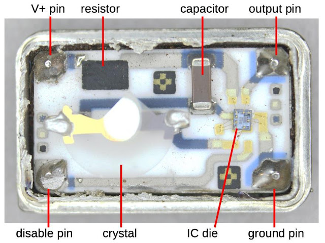
FIG: A crystal Oscillator with a steady heartbeat can - most commonly used HC-49/S (through-hole component metal package with a steel case and two leads/electrodes which flexes at a natural frequency during circuit excitation)

FIG: SMD package can with 25MHz stable output of the crystal when fed to a PLL (Phase Locked Loop). PLL can multiply it up to multi-GHz frequency clock with better vibration and temperature stability than a through-hole can. It has an accuracy spec of ±25 ppm. 

=> 1 ppm = 1 / 1000,000​  = 0.0001%

Hence, 1kHz reading = 1000.00 Hz  ±  0.025 Hz

Thus, 1.000 ms scale of a scope means worst case reading it between range of 0.999,975 ms and 1.000,025 ms

PLL Diagram:



+++++++++++.PY++++CODE+++++DIAGRAM++++++ 

import matplotlib.pyplot as plt

from matplotlib.patches import Rectangle

import matplotlib.patches as mpatches

# Create figure

fig, ax = plt.subplots(figsize=(12,4))

ax.axis('off')

def add_box(x, y, w, h, text, fontsize=12):

    rect = Rectangle((x, y), w, h, linewidth=1.5, edgecolor='black',

                     facecolor='whitesmoke')

    ax.add_patch(rect)

    ax.text(x+w/2, y+h/2, text, ha='center', va='center', fontsize=fontsize)

# Left: crystal

add_box(0.05, 0.35, 0.18, 0.3, "Quartz\nCrystal\n25 MHz", 13)

# Middle: ASIC/FPGA

add_box(0.35, 0.35, 0.28, 0.3, "ASIC / FPGA\nPLL & Dividers", 13)

# Outputs

add_box(0.75, 0.65, 0.22, 0.22, "2 GHz\nADC Clock", 12)

add_box(0.75, 0.38, 0.22, 0.18, "250 MHz\nSystem Clock", 12)

add_box(0.75, 0.12, 0.22, 0.18, "1 kHz\nProbe‑Comp", 12)

# Draw arrows

arrowprops = dict(arrowstyle='->', lw=2, color='black')

# From crystal to FPGA

ax.annotate("", xy=(0.35,0.5), xytext=(0.23,0.5), arrowprops=arrowprops)

ax.text(0.29,0.52,"25 MHz", ha='center', fontsize=11)

# From FPGA to outputs

ax.annotate("", xy=(0.75,0.76), xytext=(0.63,0.5), arrowprops=arrowprops)

ax.text(0.69,0.78,"×80 PLL", ha='center', fontsize=10)

ax.annotate("", xy=(0.75,0.47), xytext=(0.63,0.5), arrowprops=arrowprops)

ax.text(0.69,0.49,"÷? Div", ha='center', fontsize=10)

ax.annotate("", xy=(0.75,0.21), xytext=(0.63,0.5), arrowprops=arrowprops)

ax.text(0.69,0.23,"÷25 000", ha='center', fontsize=10)

plt.tight_layout()

+++++++++++++++++++END+OF+DIAGRAM++++++++++++

FIG: An SMT package Quartz crystal usually marked 25 MHz 

FIG: Paper-thin quartz wafer ≈ 0.1mm thick crystal

FIG: SiO₂ (crystalline Silicon Dioxide) Lattice structure of a unit cell. At an ordinary temperature, α-quartz form is depicted as trigonal crystal system with space group P3₁21 or P3₂21 (the two right- or left-handed enantiomorphs). Conventional cell = hexagonal axis.

A quartz slice rings like tuning fork at its natural mechanical vibration or frequency which is 10s of megahertz; an amplifier keeps that ring going, and the oscilloscope uses the resulting ultra-stable sine wave (≈ 25 MHz) as the master timer from which all other instrument frequencies are multiplied or divided. The ultrasonic vibration stays trapped inside the wafer and doesn't reach your ear.

GOOD TO KNOW TERMINOLOGIES FOR AN OSCILLOSCOPE SAFETY

Below are the Safety Terms and Symbols for an Oscilloscope:

SEMISAGA.COM ©    |    ALL RIGHTS RESERVED